I recently purchased the textbook “Aircraft Control and Simulation” by Brian L. Stevens, Frank L. Lewis, and Eric N. Johnson1. This book covers the control and simulation of aircraft. It’s really dense and frankly hard to understand. As far as aerodynamics texts go, it’s pretty typical.

One interesting item in the appendices of the book is the source code for the simulation of an F-16. It has a flight model, based on scale model wind tunnel data. The flight model consists of a dozen lookup tables and the math equations to make it fly.
The only problem: it’s written entirely in Fortran.
The source code is available on Github.
You can play the finished project right now on itch.io
Or watch the demo on Youtube:
While I am a professional software engineer and I have worked in the aerospace industry, that doesn’t mean that I understand what I’m doing.
Table of Contents
Introduction
In previous posts on this blog2 3 4, I covered the development of a flight simulator based on the lift equation and hand-tuned parameters. This gives the game designer direct control over a lot of flight parameters. For example, you can directly choose the turn rate and the G-limit of the aircraft, allowing the designer to easily tune the corner speed. This works well for game development, since the designer, and ultimately the player, care more about these high-level parameters.
But real aircraft are designed from the other direction, starting from low-level parameters such as the size, shape, and position of airfoils. Engineers tune every aspect of the aircraft in order to reach those high-level behaviors. But every design decision has trade offs and reaching the goal for one parameter means compromising another. An airliner is designed very differently from a fighter jet because of this.
Simulating all of the low-level parameters is difficult. It’s possible to simulate air flow over the vehicle using computational fluid dynamics (CFD), but this kind of software is difficult to write and even more difficult to verify.
The F-16 flight model from the textbook does not simulate the low-level parameters, but it also doesn’t simulate the high-level parameters either. It sits somewhere in between, so it serves as a useful stepping stone from my previous projects. This project will explore more advanced flight dynamics and explain the limitations of the old flight model as well as the new one.
Aerospace Conventions
Coordinate System
Before we can write any code, we need to understand the conventions used for mathematically modeling aircraft that are used in the aerospace industry. The textbook uses aerospace conventions and to use them in this project, we must convert them to Unity conventions.
The first convention is the coordinate system axes. If you’ve ever visited a graphics programming forum, you might have seen people arguing over how the X, Y, and Z axes should be arranged in their game. Especially whether to use a right handed or left handed, and Y-up or Z-up coordinate system.
This chart by Freya Holmer5 shows the axis choices made by a variety of 3D software tools.

The aerospace industry takes a different path. The most common coordinate system for aircraft is right handed, X forward, Y right, and Z down. This is completely different from every tool shown above. The textbook defines all of it’s math using this convention.

Luckily, translating between two coordinate systems is easy. You just swap the components around and then add or remove minus signs until it all works. Every calculation made by the textbook’s code can be easily translated into Unity’s coordinate system and vice versa.
Writing functions to do this is simple:
public static Vector3 ConvertVectorToAerospace(Vector3 vector) {
    return new Vector3(vector.z, vector.x, -vector.y);
}

public static Vector3 ConvertVectorToUnity(Vector3 vector) {
    return new Vector3(vector.y, -vector.z, vector.x);
}
When translating euler angles, torque, or other angular values, one additional negation is needed:
public static Vector3 ConvertAngleToAerospace(Vector3 angle) {
    // negate when switching handedness
    return -ConvertVectorToAerospace(angle);
}

public static Vector3 ConvertAngleToUnity(Vector3 angle) {
    // negate when switching handedness
    return -ConvertVectorToUnity(angle);
}
Units
For completely inscrutable reasons, American aerospace texts (and the industry!) insist on using US customary units for everything. All math is defined with these units. Distance is measured in feet. Mass is measured in slugs.
What the hell is a slug? A slug is the unit of mass in the US system. This is the equivalent unit of the kilogram in the metric system. Remember that weight and mass are not the same thing.
\(1 \, \text{kg} * 9.81 \, \text{m/s}^2 = 9.81 \, \text{N}\) \(1 \, \text{slug} * 32.17 \, \text{ft/s}^2 = 32.17 \, \text{lb}\)Mass is the measure of how much an object resists linear force. Moment of inertia is how much the object resists rotational force or torque. The unit for moment of inertia in metric is kg-m2. Thus, the equivalent unit in customary is slug-ft2.
You want to measure how much air mass is in a given volume? That’s gonna be slugs/ft3.

Speed is mostly measured in feet per second, unless you want to know the speed of the aircraft. Then you use knots, which means nautical miles per hour. Importantly, a nautical mile is not the same as a regular mile. A regular mile is 5,280 feet. A nautical mile is ~6,076 feet or exactly 1,852 meters (???).
Do you want to know how fast your ship is sailing? Just throw out this piece of wood tied to a spool of rope. The rope has knots tied at regular intervals. Count the number of knots that unspool in a given time frame. That’s how many knots your ship is making.

Finally, temperature is measured in degrees Rankine. You know how the Kelvin scale is just the Celsius scale adjusted so that 0 Kelvin equals absolute zero? Well Rankine is the same concept applied to Fahrenheit.
\(0 \, \text{R} = \text{absolute zero} \\ 534 \, \text{R} = 75 \, \text{F} = \text{room temperature}\)How the fuck did we ever build the SR-71? 💀
Unity by convention uses metric for all physics units. The flight model in the textbook uses US customary units, so every input and output of this system has to be converted. So we have to add functions to handle converting to and from US customary units. This is easy enough since conversion is just a multiplication or division operation.
Terminology
There are several terms used in aerospace that I need to define. I have used equivalent terms in the previous project, but I will clarify them here.
Alpha (α) refers to the angle of attack.
Beta (β) refers to the angle of side slip.
Longitudinal axis is the X-axis, from tail to nose.
Normal axis is the Z- axis, the vertical axis pointing downwards.
Lateral axis is the Y-axis, or side axis, pointing right.
Phi (φ) is the aircraft’s roll around the X axis.
Theta (θ) is the aircraft’s pitch around the Y axis.
Psi (ψ) is the aircraft’s yaw around the Z axis.
P, Q, and R refer to the angular velocity around the X, Y, and Z axes respectively.
In general you will find that aerodynamics texts are allergic to good variable names. I suspect this is a form of gatekeeping. Or perhaps the authors have to pay by the letter to publish.
Air Data
Airplanes need air to fly [citation needed]. Every behavior of a plane is determined by the movement of air. Therefore it is critically important, for real and simulated planes, to be able to measure the air flowing around it.
Real planes need to measure static and dynamic air pressure to determine how fast the plane is moving. Static pressure is measured by a static pressure port. It’s the pressure that you would measure if you just lifted a pressure meter to the same altitude as the plane. Static pressure decreases with altitude.
Dynamic pressure measures the pressure added by the plane’s forward motion. This requires a pitot tube to measure. As the plane moves forward it rams air into the pitot tube and increases the pressure above the static pressure. The pitot measures the total pressure of the air. By subtracting the static pressure, we can obtain the dynamic pressure.
The static and dynamic pressures can then be used to calculate many of the variables the pilot needs to fly. Most important are the airspeed and altitude of the aircraft. Specifically, these values can be used to calculate the indicated airspeed of the aircraft. Indicated airspeed is calculated directly from the dynamic pressure.
At most subsonic speeds, the dynamic pressure of air flowing over the wings is the most important variable in flight. A plane’s performance can be defined in terms of indicated airspeed. For example, a plane may have a stall speed of 100 knots indicated airspeed. This means that no matter what altitude the plane is at, the indicated airspeed will be 100 when the plane stalls.
This is important since it gives a consistent number for the stall speed regardless of atmospheric conditions. The pressure and density of the air can vary based on weather, temperature, and other factors. So the true airspeed when a stall occurs can be very inconsistent. But as long as the pilot knows the indicated airspeed, they know how their plane will behave.
For this simulator, the calculation has to work backwards. We know the true airspeed and altitude of the plane from the velocity and position of the rigidbody. From that, we can calculate the dynamic pressure. This dynamic pressure is then used for later calculations in the flight model. Additionally, the plane’s speed in mach is calculated here as well.
The original Fortran source code is given:
  	SUBROUTINE ADC(VT,ALT,AMACH,QBAR)
  	DATA R0/2.377E-3/
  	TFAC = 1.0 - 0.703E-5 * ALT
  	T = 519.0 * TFAC
  	IF (ALT .GE. 35000.0) T= 390.0
  	RHO = R0 * (TFAC**4.14)
  	AMACH= VT/SQRT(1.4*1716.3*T)
  	QBAR = 0.5*RHO*VT*VT
C 	PS = 1715.0 * RHO * T
  	RETURN
  	END
It turns out, Fortran is actually pretty good at translating formulas. So this code is not as difficult to read as I expected.
To translate this to Unity, we create a class AirDataComputer to perform these calculations. The output of the calculation is the AirData struct.
public struct AirData {
	public float altitudeMach;
	public float qBar;
}

public class AirDataComputer {
    /// <summary>
    /// Density in slugs/ft^3
    /// </summary>
    public const float SeaLevelDensity = 2.377e-3f;
    public const float MaxAltitude = 35000.0f;

    /// <summary>
    /// Calculates air data based on velocity and altitude
    /// </summary>
    /// <param name="velocity">Velocity in ft/s</param>
    /// <param name="altitude">Altitude in ft</param>
    /// <returns>Air data</returns>
    public AirData CalculateAirData(float velocity, float altitude) {
        ...
    }
}
Here we can see where the US customary units are used. The density of air at sea level is defined in slugs/ft3. The altitude is defined in feet. Theoretically, these values could be defined using metric. But the implementation of the function depends on even more values defined in customary.
const float baseTemperature = 519.0f;    	// sea level temp in R
const float minTemperature = 390.0f;     	// minimum temp in R
const float temperatureGradient = 0.703e-5f; // gradient in R / ft

altitude = Mathf.Clamp(altitude, 0, MaxAltitude);

// calculate temperature in Rankine
float temperatureFactor = 1.0f - (temperatureGradient * altitude);
float T = Mathf.Max(minTemperature, baseTemperature * temperatureFactor);
These calculations simulate the change in atmospheric conditions at different altitudes. Particularly important is how the temperature drops at higher altitudes. The temperature gradient approximates the decreases in temperature (in Rankine) as altitude increases.
This flight model supports altitudes up to 35,000 ft. Altitudes above this are not supported. At any altitude above this, the plane will behave as if it were at 35,000 ft. This is because the temperatures at this altitude no longer consistently decrease, as it does in the lower atmosphere. A more advanced atmosphere model would need to be used.
Temperature factor does not drop below about 0.75 in this range, so the resulting temperature T does not fall below 390 R.
const float gamma = 1.4f; // ratio of specific heats
const float gasConstant = 1716.3f;
float speedOfSound = Mathf.Sqrt(gamma * gasConstant * T);
float altitudeMach = velocity / speedOfSound;
Now we can calculate the speed of sound at the plane’s current altitude and use it to find the plane’s Mach number. The speed of sound varies with density, which varies with temperature. The speed of sound is equal to the square root of the ratio of specific heat, called gamma, times the gas constant, gasConstant, times the absolute temperature, T.7
Once the speed of sound is known, calculating the Mach number is just a simple division.
const float densityPower = 4.14f;

float rho = SeaLevelDensity * Mathf.Pow(temperatureFactor, densityPower);
float qBar = 0.5f * rho * velocity * velocity;
And finally the dynamic pressure is calculated from the temperature factor. I’ll admit, I don’t understand why exactly the formula is designed this way. It seems to calculate a density factor, called rho, based solely on the temperature factor, raised to an arbitrary value, densityPower.
The NASA reference provides a similar formula using metric units and using a different arbitrary power. I guess this value is just what results from using customary🤷♂️
In any case, this gives us the two air data values we need for the rest of the simulation, dynamic pressure and mach number.
Table Interpolation
Throughout this flight model, various forms of table lookups are used to determine the aircraft’s behavior. Lookup tables are commonly used in flight simulators to represent complex curves and functions. In fact, Unity’s AnimationCurve class in the previous project is used to define a few lookup tables, such as lift coefficient.

This animation curve serves as a 1 dimensional lookup table. The input dimension is AOA and the output value is lift coefficient.
Fortran code doesn’t have the luxury of using AnimationCurves, but a simple table of values with an interpolation function is almost as powerful.
1D Lookup Table
The interpolation functions provided by the textbook look something like this:
FUNCTION LOOKUP(ALPHA, RESULT)
    REAL A(-2:9)
C
    DATA A /  .770,.241,-.100,-.416,-.731,-1.053,
    &     	-1.366,-1.646,-1.917,-2.120,-2.248,-2.229 /
C
    S = 0.2*ALPHA
    K = INT(S)
    IF(K.LE.-2) K=-1
    IF(K.GE.9) K=8
    DA = S - FLOAT(K)
    L = K + INT(SIGN(1.1,DA))
    RESULT = A(K) + ABS(DA)*(A(L)-A(K))
    RETURN
END
This function takes alpha (AOA) and uses it to lookup a value from the table. Alpha is a float that can have any value from [-10, 45]. The table “A” represents values for every 5 degree increment of alpha. Note that Fortran supports arrays with an arbitrary starting index, in this case -2. So this table supports indices in the range [-2, 9].

This first step is multiplying alpha by a scaling value to create a float S, which maps alpha to the range [-2, 9]. An integer index K is created from S and then clamped to values one less than the table’s index range. The value DA is calculated as the difference between S and K.

The value L is calculated to be one index away from K, in the same direction as S. So now we have two indices to the table, K and L, which we use to read two values from the table, A(K) and A(L). DA is then used to blend between these table values and produce the final result.

This has two effects. The first is the simplest to understand. If alpha falls within the input range of the table, L and K are selected as the closest table values. For example, if alpha is 12, the two indices would be 2 and 3. The difference between S and K would be less than 1. The values A(2) and A(3) can be read from the table and then interpolated based on the value of DA. This is a fairly normal interpolation calculation.
The other effect is what happens when alpha is outside of the input range of the table. K is guaranteed to not be the first or last index, and L is allowed to be one index off of K. L and K are still valid indices, but the value of DA may be larger than 1. This means when we interpolate between A(L) and A(K), we can extrapolate values for inputs beyond the range of the table.

This means our lookup table can handle values outside of it’s input range. But there is still a limitation. As the input value gets further away from the input range, the extrapolated values will become more and more unrealistic. This allows our plane to fly slightly outside the flight envelope of the lookup tables.
I translated this function into C# like this:
public static float ReadTable(float[] table, int i, int start) {
    return table[i - start];
}

public static (int k0, int k1, float t) GetLookUpIndex(float value, float scale, int min, int max) {
    float scaled = value * scale;
    int K0 = Mathf.Clamp((int)scaled, min, max);
    float T = scaled - K0;
    int K1 = K0 + (int)Mathf.Sign(T);

    return (K0, K1, T);
}

public static float LinearLookup(float value, float scale, float[] table, int min, int max) {
    (int k0, int k1, float kT) = GetLookUpIndex(value, scale, min + 1, max - 1);
    float T = ReadTable(table, k0, min);
    float U = ReadTable(table, k1, min);
    float result = T + Math.Abs(kT) * (U - T);
    return result;
}
GetLookUpIndex calculates K, L, and DA. These variables are renamed to k0, k1, and kT respectively.
ReadTable is a function that maps array indices to a new range, to support arbitrary starting indices like Fortran. (C# surprisingly supports this feature natively, but who actually uses that?)
LinearLookup reads the k0 and k1 values from the array and performs the interpolation. This allows us to calculate values for any input to the lookup table.
Note that the expression “T + Math.Abs(kT) * (U – T)” is effectively equivalent to Mathf.LerpUnclamped.
2D Lookup Table
All of the above code is needed to perform a one dimensional table lookup. Performing this kind of table lookup with two input dimensions is called a bilinear interpolation. Extending this to two dimensions is not that much more complicated.
The two input values to the table form a two dimensional space. Our input values form a two dimensional point. Instead of selecting two array indices K and L, we need to select four array indices. These four indices form a box around our input point. We simply perform 2 one dimensional lookups, and then interpolate between them to produce the final value.

The 2 one dimensional lookups are marked in red. The final interpolation is marked in blue.
Implementing this in C# is a simple extension of the LinearLookup function:
public static float BilinearLookup(float xValue, float xScale, float yValue, float yScale, float[,] table, int xMin, int xMax, int yMin, int yMax) {
    (int x0, int x1, float xT) = GetLookUpIndex(xValue, xScale, xMin + 1, xMax - 1);
    (int y0, int y1, float yT) = GetLookUpIndex(yValue, yScale, yMin + 1, yMax - 1);
    float T = ReadTable(table, x0, y0, xMin, yMin);
    float U = ReadTable(table, x0, y1, xMin, yMin);
    float V = T + Math.Abs(xT) * (ReadTable(table, x1, y0, xMin, yMin) - T);
    float W = U + Math.Abs(xT) * (ReadTable(table, x1, y1, xMin, yMin) - U);

    float result = V + (W - V) * Math.Abs(yT);
    return result;
}
A bilinear interpolation is a very common operation in computer graphics. This is how textures are sampled when placed on 3D geometry.
In the next section, we will see that the engine thrust calculation interpolates between the output of 2 two dimensional tables. Adding this third interpolation means this calculation is now a trilinear interpolation. Interpolating between two tables is how mipmaps are blended together in computer graphics. How neat is that?

Engine
The next system we’re going to add is the engine. In my previous project, the engine was dead simple. The player selected a throttle value from [0, 1], which is multiplied by the plane’s total thrust. This works fine for that simulation and even gives us the ability to reduce thrust to zero, so the plane becomes a glider.
However, it is not a realistic simulation of how a jet engine works. In reality, a jet engine still produces some thrust at idle throttle. And there are more factors that affect thrust output than just the throttle setting.
The thrust output of a jet engine decreases with altitude and increases with speed. As altitude increases, the air gets thinner and the jet engine becomes weaker. But as speed increases, dynamic pressure, and thus pressure in the engine, increases and the engine becomes stronger. These two effects need to be considered at the same time to find the thrust output at any given moment.

Additionally, we have to consider how jet engines behave in terms of RPM. Just like piston engines (like in a typical car), jet engines have rotating components whose speed increases with throttle. The max RPM of a jet is much higher than a piston engine, however the range of possible RPM is smaller.
The engine in an F-16 has a maximum RPM of about 14,000. This is at the maximum non-afterburner power, called military power. When throttle is reduced to the lowest setting, idle, the RPM falls to about 8,400 RPM or about 60% of the max. Planes of course do not have a transmission like a car does, so this range of RPM also covers the range of thrust needed at all stages of flight.
At idle throttle, the engine runs at 60% max RPM, but only produces 8% of max thrust. At military power, the engine runs at 100% RPM and produces 100% thrust.
Military power is selected when the pilot moves the throttle lever to 77% of it’s max setting. Pushing the throttle beyond that engages the afterburner and produces even more thrust. Setting the throttle lever to 100% is called max power. Max power provides about 57% more thrust than military power. Engine RPM does not increase when using afterburner.
A significant difference between a piston engine and a jet engine is how fast the engine can change RPM. In a car, you can put the transmission in neutral and rev the engine up and down very quickly. But a jet engine is much slower to respond to changes in throttle, regardless of how fast the pilot moves the throttle lever. Generally, it can take several seconds to go from idle to military power or vice versa.
The reasons why jet engines are slower to change RPM are complicated. The change in throttle is managed by a computer to avoid compressor stall, which can cause damage or shut down of the engine. This computer will change engine parameters slowly to avoid compressor stall or any other problems that might be caused by moving the throttle too quickly.
Power
The behavior of the jet engine is included in the textbook’s flight model. RPM is not explicitly modeled, but is abstracted as power. The pilot chooses a commanded power level and the engine’s current power setting will move towards this over time. This behavior is spring-like, thus a larger difference will cause the current power setting to change faster. It takes about 2 seconds to increase from idle to military power in this flight model.
The first step is to translate the player’s throttle setting into engine power. This is a fairly simple function that maps military power, or 77% throttle, to 50% power. Full afterburner, or 100%, is mapped to 100% power. This is called the “throttle gearing”, but don’t confuse that with a car’s gearing. It’s much simpler.
FUNCTION TGEAR(THTL) ! Power command v. thtl. relationship
    IF(THTL.LE.0.77) THEN
        TGEAR = 64.94*THTL
    ELSE
        TGEAR = 217.38*THTL-117.38
    END IF
    RETURN
END
In C#, this is translated as:
public static float CalculateThrottleGear(float throttle) {
    	// maps throttle 0 - 0.77   to power 0% - 50%
    	// maps throttle 0.77 - 1.0 to power 50% - 100%

    	float power;

    	if (throttle <= militaryPowerThrottle) {
        	power = 64.94f * throttle;
    	} else {
        	power = 217.38f * throttle - 117.38f;
    	}

    	return power;
}
Those constants might seem weird, but they just define two lines with different slopes. The two lines intersect when the throttle is 0.77.

The player’s throttle setting is used to calculate the commanded power level. The rate of change of engine power also depends on the current power level. This rate is calculated in the functions PDOT and RTAU:
FUNCTION PDOT(P3,P1) ! PDOT= rate of change of power
      IF (P1.GE.50.0) THEN ! P3= actual power, P1= power command
        IF (P3.GE.50.0) THEN
            T=5.0
            P2=P1
        ELSE
            P2=60.0
            T=RTAU(P2-P3)
        END IF
      ELSE
        IF (P3.GE.50.0) THEN
            T=5.0
            P2=40.0
        ELSE
            P2=P1
            T=RTAU(P2-P3)
        END IF
      END IF
      PDOT=T*(P2-P3)
      RETURN
END

FUNCTION RTAU(DP)
    ! used by function PDOT
    IF (DP.LE.25.0) THEN
        RTAU=1.0
        ! reciprocal time constant
    ELSE IF (DP.GE.50.0)THEN
        RTAU=0.1
    ELSE
        RTAU=1.9-.036*DP
    END IF
    RETURN
END
PDOT means power rate of change. In C#, this is translated as:
float CalculatePowerRateOfChange(float actualPower, float commandPower) {
    	// calculates how fast power output should change based on commanded power
    	float T;
    	float p2;

    	if (commandPower >= 50.0) {
        	if (actualPower >= 50.0) {
            	T = 5.0f;
            	p2 = commandPower;
        	} else {
            	p2 = 60.0f;
            	T = CalculateRTau(p2 - actualPower);
        	}
    	} else {
        	if (actualPower >= 50.0) {
            	T = 5.0f;
            	p2 = 40.0f;
        	} else {
            	p2 = commandPower;
            	T = CalculateRTau(p2 - actualPower);
        	}
    	}

    	float pdot = T * (p2 - actualPower);

    	return pdot;
}

float CalculateRTau(float deltaPower) {
    	float rTau;

    	if (dp <= 25.0) {
        	rTau = 1.0f;
    	} else if (dp >= 50.0) {
        	rTau = 0.1f;
    	} else {
        	rTau = 1.9f - 0.036f * dp;
    	}

    	return rTau;
}
Power rate of change is the velocity of the power level. The most important line is this:
float pdot = T * (p2 - actualPower);
The velocity depends on the quantity (p2 – actualPower). Let’s call this value deltaPower. A larger deltaPower means a larger velocity. This is scaled by the factor T. The complexity comes from selecting the values for p2 and T. p2 is sometimes the commandPower value. T is sometimes the result of calling CalculateRTau.
These values are selected by the if statements above. These check for two conditions, the commandedPower being above 50%, and the actualPower being above 50%. This is checking whether the afterburner is being requested, and whether the afterburner is currently active. Remember that afterburner starts at 77% throttle, but 50% power.
If the afterburner is not active, then the T is given the value of CalculateRTau. If it is active, then T is given the constant value of 5.0. This matches with our expectation of how the engine’s RPM changes. When not in afterburner, the engine RPM should change slowly, thus power changes slowly. When in afterburner, fuel flow into the afterburner can change quickly, thus power changes quickly.
If we look at the function CalculateRTau, we can see that T can vary in the range [0.1, 1.0]. This depends on deltaPower. When the engine is not in afterburner, T can be at most 1.0. In afterburner, T is 5.0. That means power can change about 5 times faster when in afterburner. When multiplied with deltaPower, pdot can be as large as 250% per second.
The smallest value of T occurs when deltaPower is 50 or greater. This occurs when actualPower is 0 and commanded power is 50%, for example. This will cause the power rate of change to be quite small at only 6% per second. Note that this is simply the instantaneous rate of change. As the actual power rises, T will become larger and the rate of change will increase.
Now the reason why p2 is used instead of commandedPower is to handle the case where commandedPower is over 50% and actualPower is below 50%, or vice versa. The pilot is requesting afterburner, but the engine has not reached military power yet. In that case, deltaPower would become very large and the simulation would change power levels too quickly. To avoid this, an arbitrary constant is chosen that is on the opposite side of 50%, but not very far.
So if the actualPower is 0%, but commandedPower is 100%, p2 is set to the value of 60. This limits deltaPower to a maximum value of 60, instead of 100. And in the case where actualPower is 100% and commandedPower is 0%, deltaPower is limited to -60.
Another behavior of this code is that CalculateRTau does not handle cases where deltaPower is negative. In this case, the function returns 1, the highest value it can return. This means that the power can decrease 10 times faster than it can increase, in the most extreme case.
I don’t know if this is an intentional effect. This may match the behavior of real jet engines, or it may be an oversight by the authors. You can play with the behavior by adding a few calls to Mathf.Abs().
The practical effect of all this is that the plane’s power will lag behind the player’s throttle setting. The pilot needs to make sure that they provide enough time for the power level to change when moving the throttle.
The HUD for this project is mostly reused from the previous flight sim project. But the throttle indicator must be updated, since it can’t show the difference between commanded power and current power.
Previously, the red bar used to show the player’s throttle setting. This worked fine since power lag was not modeled. In this project, the red bar shows the engine’s current power level. I added a triangle marker to show the commanded power setting.

As you move the throttle, you’ll see that current power level changes quickly when there is a large difference from commanded power, and it slows down as it approaches. And when the engine enters afterburner, the power level changes very quickly.
Thrust
Engine power is a fairly abstract variable in this flight model. It doesn’t really correspond to any physical variable. Once we calculate the current power, we use it to find the thrust generated by the engine. Thrust in this flight model is defined in terms of pounds-force (lbf).
Thrust is defined by a group of look up tables. Each table has two dimensions as input, mach number and altitude, and the output is thrust. This gives us different thrust values in different flight conditions. Mach is input as 0.0 to 1.0 mach, in increments of 0.2 mach. Altitude is input as 0 to 50,000 ft, in increments of 10,000 ft. In other words, the table has dimensions 6×6.
The lookup tables in this flight model correspond to idle power, military power, and max power (full afterburner). The engine’s power value is used to perform a third interpolation between the output values of these tables. This makes the thrust calculation a trilinear interpolation.
At idle throttle, the thrust output has 100% influence from the idle table. When the throttle is halfway to military power, the output has 50% influence from the idle table and 50% influence from the military table. Above military power, the output will have some influence from the military power table and the max power table.
The code to read one table in Fortran is given:
DATA A/  [IDLE TABLE OMITTED]
DATA B/  [MIL TABLE OMITTED]
DATA C/  [MAX TABLE OMITTED]
H=0.0001*ALT
I=INT(H)
IF (I.GE.5) I=4
DH=H-FLOAT(I)
RM=5.*RMACH
M=INT(RM)
IF (M.GE.5) M=4
DM=RM-FLOAT(M)
CDH=1.0-DH
These parameters are used to perform the table lookups:
TMIL= S + (T-S)*DM
IF (POW.LT.50.0) THEN
    S= A(I,M)*CDH + A(I+1,M)*DH
    T= A(I,M+1)*CDH + A(I+1,M+1)*DH
    TIDL= S + (T-S)*DM
    THRUST= TIDL + (TMIL-TIDL)*POW/50.0
ELSE
    S= C(I,M)*CDH + C(I+1,M)*DH
    T= C(I,M+1)*CDH + C(I+1,M+1)*DH
    TMAX= S + (T-S)*DM
    THRUST= TMIL + (TMAX-TMIL)*(POW-50.0)*0.02
END IF
The output of the military power table, TMIL, is always calculated. If the power level is under 50, then the idle table is calculated as well, TIDL. Otherwise the max table is calculated, TMAX. The output of the two table lookups is then interpolated again to calculate the final thrust value, THRUST.
Altogether, this forms a trilinear lookup. To translate this to C#, we call BilinearLookup twice. Then those two results are interpolated based on the power level:
float InterpolateThrust(float thrust1, float thrust2, float power) {
    float result = Mathf.LerpUnclamped(thrust1, thrust2, power * 0.02f);
    return result;
}

float CalculateThrust(float power, float altitude, float rMach) {
	float a = Mathf.Max(0, altitude);
	float m = Mathf.Max(0, rMach);

	float thrust;
	float thrustMilitary = Table.BilinearLookup(a, 0.0001f, m, 5, militaryPowerTable, 0, 6, 0, 6);

	// perform trilinear interpolation
	if (power < 50.0) {
    	float thrustIdle = Table.BilinearLookup(a, 0.0001f, m, 5, idlePowerTable, 0, 6, 0, 6);
    	thrust = InterpolateThrust(thrustIdle, thrustMilitary, power);
	} else {
    	float thrustMax = Table.BilinearLookup(a, 0.0001f, m, 5, maxPowerTable, 0, 6, 0, 6);
    	thrust = InterpolateThrust(thrustMilitary, thrustMax, power - 50.0f);
	}

	return thrust;
}
The output of this calculation is the plane’s thrust in pounds-force. A simple unit conversion allows us to apply it in newtons to a Unity rigidbody:
void UpdateThrust(float dt) {
    engine.ThrottleCommand = Throttle;
    engine.Mach = Mach;
    engine.Altitude = AltitudeFeet;

    engine.Update(dt);

    Rigidbody.AddRelativeForce(new Vector3(0, 0, engine.Thrust * poundsForceToNewtons));
}
Forces
Lift force vs Normal force
In the previous flight sim project, we calculated a plane’s lift force using the angle of attack and an AnimationCurve. This is the very core of the flight simulator and is what enables flight. The flight model from the textbook does not calculate lift force.
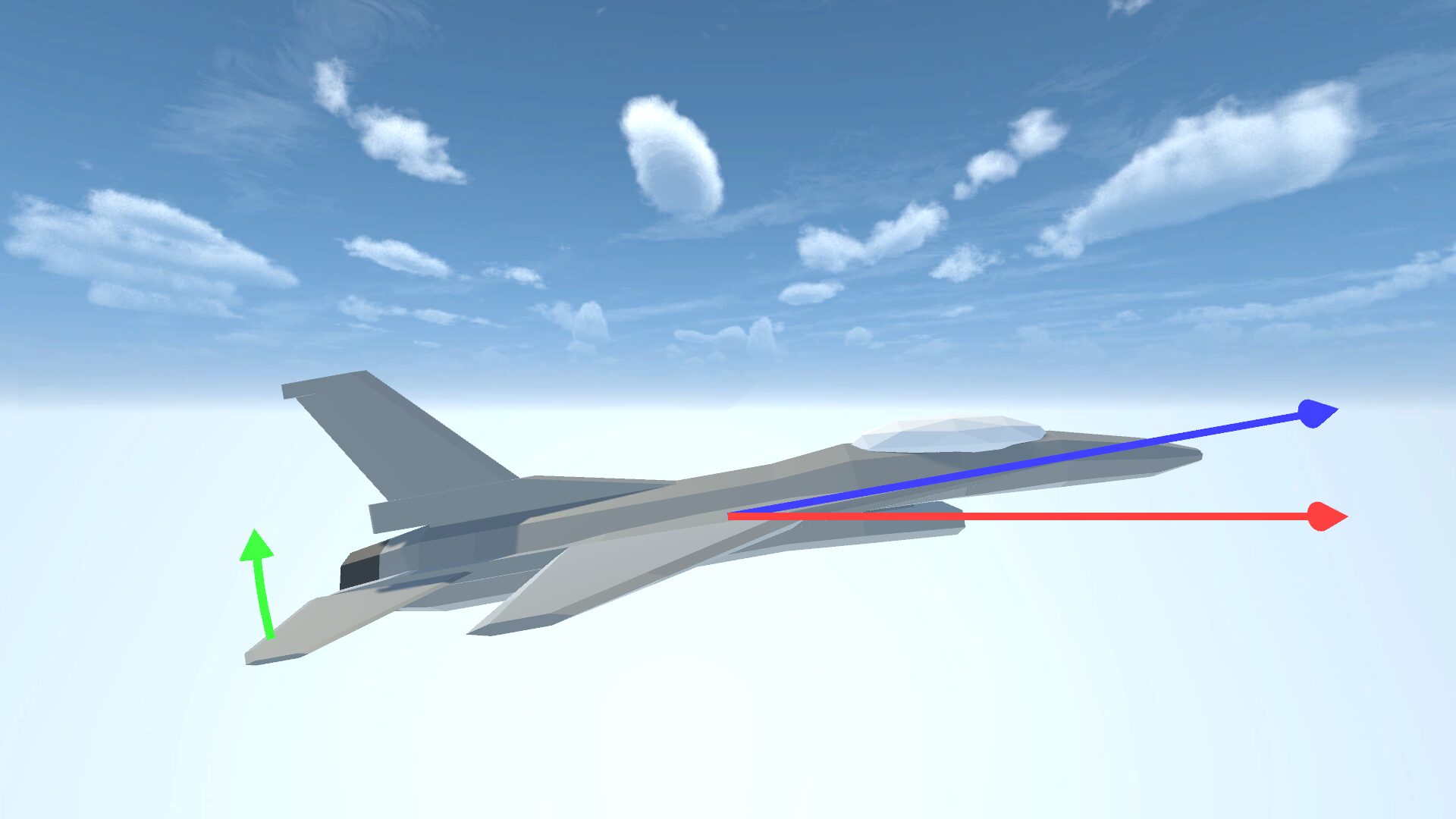
Instead what this flight model calculates is normal force. Recall that lift force is perpendicular to the aircraft’s velocity vector. Normal force is perpendicular to the aircraft’s nose. This distinction is subtle at a low angle of attack, but it becomes significant at a high angle of attack.

There are two more analogous forces to consider, drag and axial force. Drag is always exactly opposite to the aircraft’s velocity vector while axial force is opposite the aircraft’s nose. Lift and drag are perpendicular to each other and form one set of forces. Normal and axial form another perpendicular set. It’s important to understand that these two sets of forces are equally valid. In fact, they are simply the consequence of choosing different basis vectors for measuring force.
And of course there is the side force that points to the right. These forces are applied on the normal, side, and longitudinal (axial) axes, which are equivalent to the X, Y, and Z axes.

Imagine all of the forces being produced by the aircraft are summed into a single force vector. This vector would be strongly vertical, because the plane is generating enough lift to support it’s own weight, and somewhat backwards because of drag. When this vector is projected onto the lift vector, the result is the lift force. When it’s projected onto the normal vector, the result is the normal force.
Choosing to represent these forces as lift/drag or normal/axial is arbitrary. The textbook flight model only deals with normal/axial force. I suspect that’s because it’s easier to measure the physical forces when using normal/axial forces in a wind tunnel, since those are always aligned with the plane’s local axes.

The normal force is very similar to lift for low angles of attack. Lift force peaks at the stall AOA and then declines. Normal force similarly peaks at stall AOA, but it then increases again to peak at 90 AOA, with an even higher force. 90 degrees AOA means the plane is falling downwards belly first, so it’s no longer producing lift over the wings. Instead the normal vector and the drag vector are now aligned. All of the drag force projected onto the normal vector results in a large normal force.
We can calculate the lift force from the normal and axial force. Both normal and axial force may contribute to the lift force, so a complete projection needs to use both. This is the formula:
\(\text{Lift} = \text{normal} * \cos{(\text{alpha})} – \text{axial} * \sin{(\text{alpha})}\)When we apply this formula to the normal force from the textbook, this is the result:

Oh wait, that’s upside down. Recall that the Z axis points downward in this coordinate system. So a negative Z value is an upwards force. Still though, the chart is a little confusing. I inverted the values below to make it more intuitive.

We can see at 90 degrees AOA, the normal force stays relatively high while the lift force drops to zero. This roughly matches with the chart from aerospaceweb.org above.
Also note that the textbook only provides table values up to 45 degrees AOA. The extrapolation of the table lookup function is what allows us to have normal force values up to 90 degrees AOA. Additionally, the table only goes down to -10 degrees AOA. We can extrapolate further, but the data will be inaccurate by -30 degrees AOA. Large negative AOA values will quickly become inaccurate. So when you’re flying, don’t do that.
Anyways, adding these forces to our simulator is easy. The functions are fairly simple. They are called CZ, CY, and CX. These calculate the coefficients of force on the Z, Y, and X axes respectively. Note that these functions are the coefficients, not the force values themselves. They are used to calculate the force later on.
CZ or the normal coefficient is calculated like this:
FUNCTION CZ(ALPHA,BETA,EL)
    REAL A(-2:9)
C
    DATA A/ [TABLE OMITTED]
C
    S = 0.2*ALPHA
    K = INT(S)
    IF(K.LE.-2) K=-1
    IF(K.GE.9) K=8
    DA = S - FLOAT(K)
    L = K + INT(SIGN(1.1,DA))
    S = A(K) + ABS(DA)*(A(L)-A(K))
    CZ = S*(1-(BETA/57.3)**2) - .19*(EL/25.0)
C
    RETURN
END
The bulk of this code is just the table interpolation function. The table only depends on ALPHA and the output is S. The only new part here is the last line, where CZ is assigned a value. S is reduced based on the value of BETA and another term is subtracted based on EL, the elevator angle.
This is very easy to translate to C#:
float GetZAxisForceCoefficient(float alpha, float beta, float elevator) {
    	float S = Table.LinearLookup(alpha, 0.2f, zAxisTable, -2, 10);
    	float CZ = S * (1 - Mathf.Pow(beta * Mathf.Deg2Rad, 2)) - 0.19f * (elevator / 25.0f);
    	return CZ;
}
CY or the side coefficient is even simpler. It doesn’t even have a lookup table. Side force is perpendicular to both normal and axial force.
FUNCTION CY(BETA,AIL,RDR)
    CY = -.02*BETA + .021*(AIL/20.0) + .086*(RDR/30.0)
C
    RETURN
END
Side coefficient depends solely on beta, aileron angle, and rudder angle.
In C#:
float GetYAxisForceCoefficient(float beta, float aileron, float rudder) {
    float CY = -0.02f * beta + 0.021f * (aileron / 20.0f) + 0.086f * (rudder / 30.0f);
    return CY;
}
CX or the axial coefficient is basically what creates drag on the aircraft. This function is a little more complicated since it performs a bilinear interpolation, with alpha and elevator angle as the inputs.
FUNCTION CX(ALPHA,EL)
    REAL A(-2:9,-2:2)
C
    DATA A/ [TABLE OMITTED]
C
    S = 0.2*ALPHA
    K = INT(S)
    IF(K.LE.-2) K=-1
    IF(K.GE.9) K=8
    DA = S - FLOAT(K)
    L = K + INT(SIGN(1.1,DA))
    S = EL/12.0
    M = INT(S)
    IF(M.LE.-2) M=-1
    IF(M.GE.2) M=1
    DE = S - FLOAT(M)
    N = M + INT(SIGN(1.1,DE))
    V = A(K,M) + ABS(DA)*(A(L,M)-A(K,M))
    W = A(K,N) + ABS(DA)*(A(L,N)-A(K,N))
    CX = V + (W-V)*ABS(DE)
C
    RETURN
END
Thanks to the table lookup functions, this is easy to translate to C#:
float GetXAxisForceCoefficient(float alpha, float elevator) {
    float result = Table.BilinearLookup(alpha, 0.2f, elevator, 1f / 12f, xAxisTable, -2, 9, -2, 2);
    return result;
}
These three functions define all of the linear force coefficients applied to the aircraft during flight. None of these will rotate the aircraft. That is handled by a different and more complicated set of calculations.
Moments
Moment is another word for torque. (There is a subtle difference, but who cares?🤓) The F-16 flight model uses another set of look up tables to compute the moment for the aircraft.
In the previous flight sim, torque was not actually calculated. Instead, the flight model calculates the angular acceleration directly. This ignores the mass of the plane when applying the torque. This is a simplification. A more realistic flight model would take into account the mass of the aircraft when applying torque.
Note that mass is not sufficient to model rotations. When it comes to rotation, the analogy to mass is called moment of inertia. Just like mass is the property that measures an object’s resistance to force, moment of inertia is the resistance to torque. But unlike mass, moment of inertia can differ on all 3 axes. This means a torque on the X axis will result in a different angular acceleration than the same torque on the Y axis, for example.
Moment of inertia is a four-dimensional value, called AXX, AYY, AZZ, and AXZ in the textbook code. This flight model contains it’s own calculations for angular velocity using these moment of inertia values.
The flight model contains several functions that calculate the moment of the aircraft. The three basic functions are called CM, CL, and CN. These calculate the moments around the Y, X, and Z axes, AKA pitch, roll, and yaw, respectively. (L stands for longitudinal, which is the X axis. N stands for normal, which is the Z axis. M stands for… something)
These functions are all simple look up tables. CM (pitch) uses alpha and elevator angle as the input. CL (roll) and CN (yaw) use alpha and beta as the input. CM is basically the same as the other lookup table functions. CL and CN are similar to each other since they both use a symmetric table. This is because the plane is symmetric on the lateral axis, so a single table can represent the left and right sides. Their final output is then multiplied by the sign of beta.
FUNCTION CL(ALPHA,BETA)
    REAL A(-2:9,0:6)
    DATA A/    [DATA OMITTED]

    S = 0.2*ALPHA
    K = INT(S)
    IF(K.LE.-2) K=-1
    IF(K.GE.9) K=8
    DA = S - FLOAT(K)
    L = K + INT(SIGN(1.1,DA))
    S = .2*ABS(BETA)
    M = INT(S)
    IF(M.EQ.0) M=1
    IF(M.GE.6) M=5
    DB = S - FLOAT(M)
    N = M + INT(SIGN(1.1,DB))
    T = A(K,M)
    U = A(K,N)
    V = T + ABS(DA)*(A(L,M) - T)
    W = U + ABS(DA)*(A(L,N) - U)
    DUM = V + (W - V) * ABS(DB)
    CL = DUM + SIGN(1.0,BETA)

    RETURN
END
Note that there is an error in the textbook code. The final operation “CL = DUM + SIGN(…)” should use multiplication instead of addition. Otherwise this operation doesn’t make any sense.
When translated into C#:
float GetYAxisMoment(float alpha, float elevator) {
    float result = Table.BilinearLookup(alpha, 0.2f, elevator, 1f / 12f, yMomentTable, -2, 9, -2, 2);
    return result;
}

float GetXAxisMoment(float alpha, float beta) {
    float DUM = Table.BilinearLookup(alpha, 0.2f, Mathf.Abs(beta), 0.2f, xMomentTable, -2, 9, 0, 7);
    float CL = DUM * Mathf.Sign(beta);

    return CL;
}

float GetZAxisMoment(float alpha, float beta) {
    float DUM = Table.BilinearLookup(alpha, 0.2f, Mathf.Abs(beta), 0.2f, zMomentTable, -2, 9, 0, 7);
    float CL = DUM * Mathf.Sign(beta);

    return CL;
}
Notice that CM takes “elevator” as an argument, so this is where the elevator’s turning effect is calculated. But CL and CN do not take any control surface as an argument. These functions only apply moment based on alpha and beta. For example, at high angles of sideslip, the plane tends to roll. On real planes, this is caused by wing sweep. In this flight model, it’s caused by the CL function.
Elevators are applied in CM, but rudder and ailerons are not. Those are actually handled by four more functions, called DLDA, DLDR, DNDA, and DNDR. The names are cryptic, but it just means which axis is affected from which control surface.
The “L” stands for longitudinal, so DLDA is the longitudinal moment from the ailerons, A. DLDR is the longitudinal moment from the rudder, R. The “N” stands for normal, so those functions are the normal axis moment from aileron and rudders.
These four functions are eventually summed with the CL and CN functions above. These functions mean that roll is affected by aileron and rudder, and yaw is affected by aileron and rudder.
Damping
There is one more set of coefficients that must be calculated. These are the damping coefficients and they depend solely on alpha. These values are stored in 9 distinct 1D lookup tables. The code for these lookups is the same as the other lookup code.
These values are stored in an array of length 9 called D.
Damping is the moment that opposes the angular velocity of an aircraft, essentially angular drag. They affect the other moment values in somewhat complex ways. For example, some of them are combined with the plane’s current bank value to affect the roll moment.
What isn’t clear is what the damping values actually represent. In the C# code, I added these comments explaining their meaning:
//  D[0] = CXq
//  D[1] = CYr
//  D[2] = CYp
//  D[3] = CZq
//  D[4] = Clr
//  D[5] = Clp
//  D[6] = Cmq
//  D[7] = Cnr
//  D[8] = Cnp
Hope this helps!
The best I can tell is that “CXq” is the damping moment on the X axis relative to q, which is the angular velocity around the Y axis. The other damping values follow this naming scheme.
This is yet another example of aerodynamics texts with poor variable names.
Complete Flight Model
With all of the individual coefficients defined, we can now implement the complete flight model for the F-16. This flight model actually contains it’s own physics integrator. The text provides it’s own code for calculating velocity and angular velocity from the aerodynamic forces.
Strictly speaking, we don’t need to use this code since Unity allows us to provide those same forces and then performs the physics calculation for us. Setting the mass is easy enough, we just have to convert slugs to kilograms. The textbook code calculates acceleration by dividing the force by the aircraft mass. We simply omit this division, convert the forces to newtons, and apply it to the rigidbody.
However the moment of inertia is more complicated. The textbook provides the 4 dimensional MOI values, but Unity expects a 3 dimensional inertia tensor. That inertia tensor is then rotated by a quaternion called “inertiaTensorRotation”. I have no idea how to calculate this quaternion from the textbook’s provided value.
Therefore, we continue to use the textbook’s code for applying moment and simply apply the resulting angular acceleration to the rigidbody.
The Fortran code for the flight model is concise, yet scrutable. The first step is to read the plane’s current state from the input state vector X. This is simply an array that contains all of the relevant data for this frame.
VT= X(1); ALPHA= X(2)*RTOD; BETA= X(3)*RTOD
PHI=X(4); THETA= X(5); PSI= X(6)
P= X(7); Q= X(8); R= X(9); ALT= X(12); POW= X(13)
VT is the plane’s velocity in feet per second.
ALPHA and BETA are the plane’s AOA and AOS in degrees. RTOD is the constant to convert from radians to degrees.
PHI, THETA, and PSI are the plane’s roll, pitch, and yaw in radians.
P, Q, and R are the plane’s angular velocities (or roll rate, pitch rate, and yaw rate) in radians per second.
ALT is the altitude in feet.
POW is the current power level of the engine (0 – 100).
The air data computer (ADC) and engine model are then called using these variables:
CALL ADC(VT,ALT,AMACH,QBAR); CPOW= TGEAR(THTL)
XD(13) = PDOT(POW,CPOW); T= THRUST(POW,ALT,AMACH)
The ADC function populates the variables AMACH and QBAR, which are the altitude mach and dynamic pressure.
CPOW is the pilot’s commanded power setting. That is, the power level returned by calling the throttle gear function, TGEAR, on the throttle lever position, THTL.
The array XD is the output state vector. Specifically, it holds the calculated derivative for every input value. XD(13) is set to the value calculated by PDOT, which is the velocity of the power level.
T is the thrust in pounds-force output by the engine, calculated using the power level, altitude, and altitude mach.
Then the aerodynamic coefficients are calculated using the force and moment functions:
  CXT = CX (ALPHA,EL)
  CYT = CY (BETA,AIL,RDR)
  CZT = CZ (ALPHA,BETA,EL)
  DAIL= AIL/20.0; DRDR= RDR/30.0
  CLT = CL(ALPHA,BETA) + DLDA(ALPHA,BETA)*DAIL
 &                 	+ DLDR(ALPHA,BETA)*DRDR
  CMT = CM(ALPHA,EL)
  CNT = CN(ALPHA,BETA) + DNDA(ALPHA,BETA)*DAIL
 &                 	+ DNDR(ALPHA,BETA)*DRDR
The values CXT, CYT, and CZT are the coefficients on the X, Y, and Z axes, calculated by calling their respective coefficient functions.
EL, AIL, and RDR are the current position of the elevators, ailerons, and rudder in degrees. DAIL and DRDR are simply the angle of these surfaces divided by the max angle. Their range is [-1, 1].
The values CLT, CMT, and CNT are the moment coefficients on the longitudinal, m’lateral, and normal axes. Note that CM calculates moment caused by the elevator position. The effects of the other control surfaces are calculated in the DLDA, DLDR, DNDA, and DNDR functions.
Then some other values are calculated and the damping coefficients are added to the above values:
TVT= 0.5/VT; B2V= B*TVT; CQ= CBAR*Q*TVT
CALL DAMP(ALPHA,D)
CXT= CXT + CQ * D(1)
CYT= CYT + B2V * ( D(2)*R + D(3)*P )
CZT= CZT + CQ * D(4)
CLT= CLT + B2V * ( D(5)*R + D(6)*P )
CMT= CMT + CQ * D(7) + CZT * (XCGR-XCG)
CNT= CNT + B2V*(D(8)*R + D(9)*P) - CYT*(XCGR-XCG) * CBAR/B
I’ll be honest, I straight up don’t know what any of these values are or why they are being applied like this. The effect appears to be angular damping (AKA angular drag) which opposes the plane’s angular velocity.
The value (XCGR – XCG) is the center of gravity reference minus the current center of gravity. This allows us to alter the center of gravity of the aircraft and see how that affects stability.
XCGR is 0.35 for this flight model. XCG is 0.35 by default. XCG is the normalized position of the center of gravity, with a possible range of [0, 1]. This means that when XCG is 0.35, the term (XCGR – XCG) becomes zero and the aircraft is balanced around it’s center of gravity.
The center of gravity term affects CMT and CNT, which are the pitch and yaw axes. The roll axis is not affected.
The next block of code is fun:
CBTA = COS(X(3)); U=VT*COS(X(2))*CBTA
V= VT * SIN(X(3)); W=VT*SIN(X(2))*CBTA
STH = SIN(THETA); CTH= COS(THETA); SPH= SIN(PHI)
CPH = COS(PHI) ; SPSI= SIN(PSI); CPSI= COS(PSI)
QS = QBAR * S ; QSB= QS * B; RMQS= QS/MASS
GCTH = GD * CTH ; QSPH= Q * SPH
AY = RMQS*CYT ; AZ= RMQS * CZT
This writhing mass of arithmetic is simply pre-calculating a lot of the values that are used to calculate the aerodynamic forces. Some of these values are used in multiple places, so to avoid repeating them, they are pulled out of those equations and placed here.
This is essentially the “common subexpression” optimization pass of a compiler, but applied manually.
The important variables are U, V, and W, which is the plane’s velocity on the X, Y, and Z axes respectively.
QS is QBAR (dynamic pressure) times S (wing area).
Now the aerodynamic forces are calculated:
UDOT = R*V - Q*W - GD*STH + (QS * CXT + T)/MASS
VDOT = P*W - R*U + GCTH * SPH + AY
WDOT = Q*U - P*V + GCTH * CPH + AZ
DUM = (U*U + W*W)
xd(1) = (U*UDOT + V*VDOT + W*WDOT)/VT
xd(2) = (U*WDOT - W*UDOT) / DUM
xd(3) = (VT*VDOT- V*XD(1)) * CBTA / DUM
Once again, I don’t actually understand what I’m reading. UDOT etc are the accelerations on each axis. These values are then used to update the output state vector xd(1), xd(2), and xd(3), which are the VT, ALPHA, and BETA that will be used in the next frame.
It appears that this flight model is calculating the change in alpha and beta directly from the change in velocity. This is not necessary in C#, since we can calculate alpha and beta fresh in each frame.
But I don’t fully understand how UDOT is calculated. R and Q are angular velocities, so multiplying them with linear velocity doesn’t make any sense. Perhaps this is some physics equation that I’m not familiar with.
GD * STH is the gravity acceleration times sin(theta). This is simply how gravity is applied. When the plane is level (theta = 0), sin(theta) is 0. The plane experiences no gravity acceleration on the X axis (the forward axis). When the plane is pointed straight down, sin(theta) = 1, so the plane experiences the full force of gravity pulling on the X axis.
A similar calculation is made for every axis.
For UDOT, the final term is (QS * CXT + T) / MASS. This is the coefficient CXT plus the thrust from the engine, divided by mass. VDOT and WDOT have similar final terms, made more difficult to read by the common subexpression optimization.
Ignoring the other terms, the 3 accelerations can be written:
UDOT = (QS * CXT + T)/MASS
VDOT = AY
WDOT = AZ
Then the variables can be expanded and rewritten:
UDOT = (QBAR * S * CXT + T) / MASS
VDOT = (QBAR * S * CYT)     / MASS
WDOT = (QBAR * S * CZT)     / MASS
This is simply the force coefficient times QBAR (dynamic pressure) times S (wing area). Then thrust is added to the X axis. This is how all forces are applied to the aircraft.
Recall the lift equation from my previous project:
\(L=\frac12\times A\times\rho\times C_L\times v^2\)- L is the resulting lift force
- A is the surface area
- ρ (rho) is the air density
- CL is the coefficient of lift
- v is the velocity
The surface area A is equivalent to the wing area S in the Fortran code. CL is equivalent to the variables CXT, CYT, or CZT. The factor ρ * v2 is equivalent to QBAR. Thus we are essentially calculating a lift force on all three axes. But remember that we are specifically calculating normal force, not lift force.
The roll, pitch, and yaw state vectors are then updated:
xd(4) = P + (STH/CTH)*(QSPH + R*CPH)
xd(5) = Q*CPH - R*SPH
xd(6) = (QSPH + R*CPH)/CTH
Once again, these equations make zero sense to me🤷♂️. It’s important for the Fortran code, but we will be calculating roll, pitch, and yaw differently in C#.
Aerodynamic moment is about to be calculated. However this depends on the moment of inertia values and some more values derived from those:
PARAMETER (AXX=9496.0, AYY= 55814.0, AZZ=63100.0, AXZ= 982.0)
PARAMETER (AXZS=AXZ**2, XPQ=AXZ*(AXX-AYY+AZZ),GAM=AXX*AZZ-AXZ**2)
PARAMETER (XQR= AZZ*(AZZ-AYY)+AXZS, ZPQ=(AXX-AYY)*AXX+AXZS)
PARAMETER ( YPR= AZZ - AXX )
Now the aerodynamic moment is calculated:
ROLL  = QSB*CLT
PITCH = QS *CBAR*CMT
YAW   = QSB*CNT
PQ    = p*Q
QR    = Q*R
QHX   = Q*HX
xd(7) = ( XPQ*PQ - XQR*QR + AZZ*ROLL + AXZ*(YAW + QHX) )/GAM
xd(8) = ( YPR*P*R - AXZ*(P**2 - R**2) + PITCH - R*HX )/AYY
xd(9) = ( ZPQ*PQ - XPQ*QR + AXZ*ROLL + AXX*(YAW + QHX) )/GAM
There’s a lot of stuff going on here. The output state vectors are updated using the moment of inertia values as well as HX, which is the angular momentum of the spinning engine mass. I don’t know enough about physics to fully understand why these equations are defined like this.
But we can at least see how the moment coefficients are used if we expand the ROLL, PITCH, and YAW variables:
ROLL  = QBAR * S * B    * CLT
PITCH = QBAR * S * CBAR * CMT
YAW   = QBAR * S * B    * CNT
ROLL and YAW depend on B, the wingspan of the plane. Pitch depends on CBAR, the mean aerodynamic chord.
The final step is to calculate the world space position of the aircraft. Since we are using Unity rigidbodies to implement the flight model, this step is not translated to C#. But for reference:
T1= SPH * CPSI; T2= CPH * STH; T3= SPH * SPSI
S1= CTH * CPSI; S2= CTH * SPSI; S3= T1 * STH - CPH * SPSI
S4= T3 * STH + CPH * CPSI; S5= SPH * CTH; S6= T2*CPSI + T3
S7= T2 * SPSI - T1; S8= CPH * CTH

xd(10) = U * S1 + V * S3 + W * S6 ! North speed
xd(11) = U * S2 + V * S4 + W * S7 ! East speed
xd(12) = U * STH -V * S5 - W * S8 ! Vertical speed

AN = -AZ/GD; ALAT= AY/GD;
Now we can start translating this into C# using Unity’s physics engine to replace some parts.
A lot of the code can be reused from the previous flight sim project. Using it for this new flight model only requires some conversion into customary units and back. The main class that controls everything is Plane. This class contains instances of the AirDataComputer, Engine, and Aerodynamics, which is where the translated Fortran code lives.
One simplification can be made since we are using Unity physics. We do not need to calculate the acceleration of the aircraft manually. That can be done automatically by the physics engine. However, the moment calculation needs to be copied more or less directly from the textbook.
The air data computer needs to be called:
void UpdateAirData() {
    float speed = LocalVelocity.magnitude;  // m/s
    float speedFeet = speed * metersToFeet;
    AltitudeFeet = Rigidbody.position.y * metersToFeet;

    airData = airDataComputer.CalculateAirData(speedFeet, AltitudeFeet);
}
Then the engine needs to be updated and the thrust force applied:
void UpdateThrust(float dt) {
    engine.ThrottleCommand = Throttle;
    engine.Mach = Mach;
    engine.Altitude = AltitudeFeet;

    engine.Update(dt);

    Rigidbody.AddRelativeForce(new Vector3(0, 0, engine.Thrust * poundsForceToNewtons));
}
For the aerodynamics class, a struct with all relevant aerodynamic state is passed, similar to the state vector in the Fortran code.
public struct AerodynamicState {
    public Vector4 inertiaTensor;
    public Vector3 velocity;
    public Vector3 angularVelocity;
    public AirData airData;
    public float altitude;
    public float alpha;
    public float beta;
    public float xcg;
    public ControlSurfaces controlSurfaces;
}
This is populated by the Plane class, which also handles unit conversions:
AerodynamicState currentState = new AerodynamicState {
    inertiaTensor = inertiaTensor,
    velocity = ConvertVectorToAerospace(LocalVelocity) * metersToFeet,
    angularVelocity = ConvertAngleToAerospace(LocalAngularVelocity),
    airData = airData,
    alpha = alpha,
    beta = beta,
    xcg = centerOfGravityPosition,
    controlSurfaces = ControlSurfaces
};

var newState = aerodynamics.CalculateAerodynamics(currentState);
All of the flight model code is located inside the Aerodynamics class.
First step is to call the aerodynamic coefficient functions from above:
Vector3 GetForceCoefficient(float alpha, float beta, float aileron, float rudder, float elevator) {
    return new Vector3(
        GetXAxisForceCoefficient(alpha, elevator),
        GetYAxisForceCoefficient(beta, aileron, rudder),
        GetZAxisForceCoefficient(alpha, beta, elevator)
    );
}

Vector3 GetMomentCoefficient(float alpha, float beta, float elevator) {
    return new Vector3(
        GetXAxisMomentCoefficient(alpha, beta),
        GetYAxisMomentCoefficient(alpha, elevator),
        GetZAxisMomentCoefficient(alpha, beta)
    );
}

...

public AerodynamicForces CalculateAerodynamics(AerodynamicState currentState) {
    Vector3 forceCoefficient = GetForceCoefficient(
        currentState.alpha, currentState.beta,
        currentState.controlSurfaces.aileron, currentState.controlSurfaces.rudder, currentState.controlSurfaces.elevator
    );

    Vector3 momentCoefficient = GetMomentCoefficient(
        currentState.alpha, currentState.beta, currentState.controlSurfaces.elevator
    );
}
Then we calculate the damping values. This function simply performs the 9 table lookups.
void CalculateDampingValues(float alpha) {
    float S = 0.2f * alpha;
    int K = Mathf.Clamp((int)S, -1, 8);

    float DA = S - K;
    int L = K + (int)Mathf.Sign(DA);

    for (int i = 0; i < 9; i++) {
        dampingTable[i] = ReadDampTable(dampTable, K, i) + Math.Abs(DA) * (ReadDampTable(dampTable, L, i) - ReadDampTable(dampTable, K, i));
    }
}
Then the variables we need later are calculated:
// calculate variables
float P = currentState.angularVelocity.x;   // roll rate
float Q = currentState.angularVelocity.y;   // pitch rate
float R = currentState.angularVelocity.z;   // yaw rate

float airspeed = Mathf.Max(1, currentState.velocity.magnitude);
float TVT = 0.5f / airspeed;

float B2V = wingSpanFt * TVT;
float CQ = CBAR * Q * TVT;

float DAIL = currentState.controlSurfaces.aileron / 20.0f;
float DRDR = currentState.controlSurfaces.rudder / 30.0f;

float QS = currentState.airData.qBar * wingAreaFtSquared;
float QSB = QS * wingSpanFt;
Then damping is applied to the force and moment coefficients:
// damping
float CXT = forceCoefficient.x + CQ * dampingTable[0];
float CYT = forceCoefficient.y + B2V * (dampingTable[1] * R + dampingTable[2] * P);
float CZT = forceCoefficient.z + CQ * dampingTable[3];

float CLT = momentCoefficient.x + B2V * (dampingTable[4] * R + dampingTable[5] * P);
CLT += GetDLDA(currentState.alpha, currentState.beta) * DAIL;
CLT += GetDLDR(currentState.alpha, currentState.beta) * DRDR;
float CMT = momentCoefficient.y + CQ * dampingTable[6] + CZT * (XCGR - currentState.xcg);
float CNT = momentCoefficient.z + B2V * (dampingTable[7] * R + dampingTable[8] * P) - CYT * (XCGR - currentState.xcg) * CBAR / wingSpanFt;
CNT += GetDNDA(currentState.alpha, currentState.beta) * DAIL;
CNT += GetDNDR(currentState.alpha, currentState.beta) * DRDR;
Note that the damping array in Fortran is 1 based, while the same array in C# is 0 based.
Forces are calculated from the force coefficients. Since we are using Unity’s physics to apply gravity, the gravity terms are not included here. The force from engine thrust is applied outside of this class. And force is applied to a rigidbody, so acceleration does not need to be calculated manually. So the force calculations are now very simple:
// forces
// Acceleration in original text. Need to calculate force instead of acceleration
float UDOT = QS * CXT;
float VDOT = QS * CYT;
float WDOT = QS * CZT;
Moments are calculated using largely the same code as the textbook:
// moments
float ROLL = QSB * CLT;
float PITCH = QS * CBAR * CMT;
float YAW = QSB * CNT;
float PQ = P * Q;
float QR = Q * R;
float QHX = Q * HX;

// calculate inertia values
float AXX = currentState.inertiaTensor.x;
float AYY = currentState.inertiaTensor.y;
float AZZ = currentState.inertiaTensor.z;
float AXZ = currentState.inertiaTensor.w;

float AXZS = AXZ * AXZ;
float XPQ = AXZ * (AXX - AYY + AZZ);
float GAM = AXX * AZZ - AXZS;
float XQR = AZZ * (AZZ - AYY) + AXZS;
float ZPQ = (AZZ - AYY) * AXX + AXZS;
float YPR = AZZ - AXX;

float rollAccel  = ((XPQ * PQ)	- (XQR * QR) + (AZZ * ROLL) + (AXZ * (YAW + QHX))) / GAM;
float pitchAccel = ((YPR * P * R) - (AXZ * (P * P - R * R))   + PITCH - (R * HX))	/ AYY;
float yawAccel   = ((ZPQ * PQ)	- (XPQ * QR) + (AXZ * ROLL) + (AXX * (YAW + QHX))) / GAM;
Finally, the force and angular acceleration is returned:
public AerodynamicForces CalculateAerodynamics(AerodynamicState currentState) {
    ...
    result.force = new Vector3(UDOT, VDOT, WDOT);
    result.angularAcceleration = new Vector3(rollAccel, pitchAccel, yawAccel);

    return result;
}
Then in the Plane class, the force and angular acceleration can be applied to the rigidbody:
// aeroForces in pounds
var forces = ConvertVectorToUnity(aeroForces) * poundsForceToNewtons;
Rigidbody.AddRelativeForce(forces);

// aeroAngularAcceleration changes angular velocity directly
Vector3 avCorrection = ConvertAngleToUnity(aeroAngularAcceleration);
Rigidbody.AddRelativeTorque(avCorrection, ForceMode.Acceleration);
lastAngularAcceleration = avCorrection;
The plane is now able to fly. But if you try flying it right now, you will quickly find that it is impossible to fly by hand.
Stability
One important aerodynamic effect not modeled in my previous flight sim project is stability. Stability is the behavior of an aircraft when it’s disturbed from it’s flight path. More specifically, it’s how the aircraft behaves when it’s nose vector doesn’t match it’s velocity vector. Stability is the force that pulls the nose vector back towards the velocity vector.
For most aircraft, stability is created by the stabilizers in the tail. A stabilizer is simply a small airfoil (wing). Even without the pilot giving input, the stabilizers act like the fins of a dart. As the plane increases it’s Angle of Attack, the horizontal stabilizer will produce a lift force at the rear of the plane. This creates a torque that pulls the plane’s nose back towards the velocity vector, thus reducing the AOA. Likewise, the vertical stabilizers will create a torque that reduces Angle of Slip.
Keep in mind that stability depends on AOA, just as lift does. When the aircraft has a large AOA, the wings produce lift, which brings the velocity vector towards the nose vector. The stabilizers create torque which brings the nose vector towards the velocity vector. These two forces balance out somewhere and the aircraft will take a new attitude with a new velocity.

However, the aircraft needs to maintain a non-zero AOA to create enough lift to fly straight and level. How does it maintain this AOA when stability works to reduce AOA to zero? The stabilizers can be trimmed to hold a specific AOA. This means that the stabilizers produce zero torque at this particular non-zero AOA. In some planes this must be done manually by the pilot, but in the F-16 this is done automatically by the FCS.

The two forces of lift and stability combine to produce the “feel” of an aircraft’s controls. The tendency for the nose to be pulled towards the velocity vector is called positive stability. Most non-fighter aircraft are designed to have positive stability to maximize safety and ease of flying.
But fighter aircraft like the F-16 are different. These aircraft are often designed to have neutral or even negative stability. Neutral stability means that the aircraft will hold it’s current attitude. Negative stability means that the aircraft will rotate even further away from the velocity vector, at an increasing rate.
The previous flight sim does not model this at all. There is no torque that changes the plane’s attitude except for the steering force. So the behavior is best described as neutrally stable.
This F-16 flight model does include stability. But keep in mind that the real F-16 was designed to have relaxed static stability. This means that it is positively stable, but weakly so. This makes the aircraft more maneuverable and better at retaining energy while turning. But flying an aircraft like this is difficult or even impossible for a human pilot. The plane will depart from steady flight from the smallest stick input or wind gust. The only way a human can handle an aircraft like this during long and stressful missions is with a computerized flight control system.
Flight Control System
A flight control system (FCS) is a computer located between the flight stick and the control surfaces. This computer translates the pilot’s input on the flight stick into control surface movement. It can react to disturbances in the plane’s attitude more quickly and precisely than a human can.
In my previous flight sim project, the control surfaces were purely cosmetic. The actual method used to turn the vehicle was by applying torque directly to the center of mass. That torque was calculated to create a certain amount of angular acceleration without exceeding the plane’s turn rate limit.
For example, the plane had a turn rate on the pitch axis of 60 degrees per second and an acceleration of 120 degrees per second per second. The plane’s turn rate never leaves the range [-60, 60]. Actually, no torque is ever calculated. Unity provides a function to apply angular acceleration directly, ignoring moment of inertia. I chose this behavior to make it easy to both understand the code and to fly the plane.
But this F-16 simulator does depend on the position of the control surfaces. Instead of specifying the acceleration directly, this simulator specifies the torque (moment) and calculates the resulting acceleration. This is more accurate to how serious simulators work and how real planes fly, but this makes controlling the plane more difficult.
The steering system in the previous flight sim project was essentially a perfect FCS that could always achieve the turn rate chosen by the pilot. This is helped by the fact that that simulator does not model aerodynamic stability or instability at all. Spinning out of control was simply not possible.
This F-16 simulator is more difficult to control both because of the more accurate control surfaces and because of the modeled stability. You can actually try to fly this F-16 manually, by disabling the FCS in the config menu.
You will quickly find that the F-16 is almost impossible to fly manually. Every small disturbance from straight and level flight will create small torques that turn your plane unexpectedly. If you try to correct it with the control stick, you will almost certainly overcorrect and send the plane into a new and exciting attitude. This is called pilot induced oscillation.

It simply isn’t possible for a human to react quickly and precisely enough to fly this aircraft. You may be able to fly straight and level with some effort, but you will quickly lose control if you attempt any maneuver. This is indeed a property of the real F-16.
The textbook provides no Fortran code for the FCS. From here on out, it’s my own original code.
PID Controllers
The steering system from the previous project cannot be reused. The solution is to use PID controllers, a topic I’ve covered on this blog before.11
To be more specific, steering in the previous flight sim was easy because we could read the angular velocity of the aircraft and apply a torque that directly countered any undesired movement. This F-16 flight model does not allow us to apply torques directly. We can only set the angle of the control surfaces. This is the problem that PID controllers are good at solving.
Adding the PID controllers is simple. The pilot’s control input is used to select a target angular velocity for the plane, for the 3 axes of rotation. This is given to three independent PID controllers. The output of the PID controllers set the target position for the control surface.
The control surface positions are then passed into the flight model inside AerodynamicState.
Vector3 targetAV = Vector3.Scale(controlInput, steeringSpeed * steeringSpeedFactor);

var accel = lastAngularAcceleration * Mathf.Rad2Deg * dt;

controlSurfaceTarget = new Vector3(
    pitchController.Calculate(dt, av.x, accel.x, targetAV.x),
    -yawController.Calculate(dt, av.y, accel.y, targetAV.y),
    rollController.Calculate(dt, av.z, accel.z, targetAV.z)
);

var current = ControlSurfaces;

ControlSurfaces = new ControlSurfaces(
    Utilities.MoveTo(current.elevator, controlSurfaceTarget.x, elevatorSpeed, dt, -elevatorRange, elevatorRange),
    Utilities.MoveTo(current.rudder,   controlSurfaceTarget.y, rudderSpeed,   dt, -rudderRange, rudderRange),
    Utilities.MoveTo(current.aileron,  controlSurfaceTarget.z, aileronSpeed,  dt, -aileronRange, aileronRange)
);

...

AerodynamicState currentState = new AerodynamicState {
    controlSurfaces = ControlSurfaces
};

var newState = aerodynamics.CalculateAerodynamics(currentState);
Here the PIDs are named “pitchController”, “yawController”, and “rollController”. They are all tuned separately to handle a single axis.
When the player releases the stick, the PID controllers will attempt to hold an angular velocity of zero. This makes the aircraft feel like it’s neutrally stable. This also acts as a way to trim the aircraft, so that level flight can be maintained without needing to constantly pull the stick. The PID controller will detect an undesired rotation and move the elevators at a slight angle to counter it.
These PID controllers only add a small amount of complexity to the code, but they achieve similar results as the perfect FCS from the previous project. But there are still limitations that prevent it from being a perfect FCS.
First, the PID controllers must be tuned. The output has to be strong enough to quickly respond to pilot inputs, while avoiding oscillation. This is of course a limitation of any PID control system.
Second, the control surfaces move at a finite speed. This means that it will take some time for the control surface to match the FCS’s commands. So the commands will be imperfectly applied to the aircraft.
Third, unlike the previous flight sim, the three axes of rotation are not independent. For example, a large angle of slip will cause the plane to roll. This is due to the swept wings of the F-16. The roll controller will cancel this out somewhat, but a large enough AOS will result in an uncommanded roll.
Even with these limitations, the PID controllers work fairly well at keeping the plane in control.
Additionally, I use a technique called gain scheduling to change the gain parameters of the roll controller. Because roll performance increases with airspeed, we need a way to limit the amount of aileron movement at high speed. I add two animation curves, which take speed as input, and give the P and D gain of the roll controller as output.
rollController.P = rollPSchedule.Evaluate(Mathf.Max(0, LocalVelocity.z));
rollController.D = rollDSchedule.Evaluate(Mathf.Max(0, LocalVelocity.z));

Vector3 fcsTarget = new Vector3(
    pitchController.Calculate(dt, av.x, accel.x, targetAV.x),
    -yawController.Calculate(dt, av.y, accel.y, targetAV.y),
    rollController.Calculate(dt, av.z, accel.z, targetAV.z)
);
This allows us to change the strength of the roll controller at different speeds. A more advanced FCS might have a gain schedule for each controller, possibly using more inputs than just airspeed. In fact, if there were multiple inputs, we would need a 2D lookup table to calculate the gain schedule.
Because the flight model is a complete description of how the aircraft will respond at different combinations of AOA, AOS, and control input, it is theoretically possible to design an FCS system that perfectly counters all of the unwanted tendencies. However, that is beyond my understanding of aerodynamics and control theory.
G and AOA Limiter
The weakness of PID controllers is that they only control the angular velocity of the plane. This is not sufficient to control the plane. The previous project has a G limiter, which is simple since steering torque is applied directly to the aircraft. Adding a G limiter is more complicated with this F-16 flight model.
Additionally, a critical part of the FCS on a real F-16 is the AOA limiter. Just like the G limiter prevents the pilot from creating excessive G-forces while maneuvering, the AOA limiter prevents excessive AOA. This is because the aircraft becomes so unstable at about 28 degrees AOA that even the FCS can not compensate. And importantly, our flight model only supports a limited range of AOA (up to 45 degrees), so if the pilot goes beyond that, the behavior of the simulator becomes nonsensical. So limiting the AOA to about 25 degrees is important for maintaining stable flight.
The previous flight sim project did not have anything like an AOA limiter. I simply tuned the steering strength so that AOA would not exceed about 15 degrees (unless stalling). And even then, there is no instability caused by high AOA, so nothing bad happens if the pilot exceeds that.
We need a system that prevents the pilot from exceeding 25 degrees AOA. This would be implemented as a multiplier on the pilot’s stick input, just like a G limiter. Since there are two limits, we simply select the more restrictive limit using min(). So if the G limiter says to limit input to 0.75 and the AOA limiter says to limit input to 0.5, the value 0.5 is chosen.
Because this flight model uses lookup tables, there is no simple formula for calculating either the G limiter or AOA limiter. The G limiter from the previous project won’t work here. Additionally, the relationship between steering input and AOA is not simple. There is a feedback loop between AOA and lift. As AOA increases, lift increases. But as lift increases, AOA decreases since lift pulls the plane onto a new velocity vector. Not to mention lift also depends on airspeed and altitude.
Luckily, the F-16 flight model is completely disconnected from Unity’s physics system. We can actually run the flight model as much as we want with any inputs, and use the outputs for any purpose. There is the “main” flight model that syncs with a Unity rigidbody. But we can create “side” flight models to predict future behavior of the plane.
I chose to implement the G and AOA limiters by running a side flight model. This side model takes the pilot’s inputs and simulates the aircraft in a simplified world state. In a single physics update, the main flight model runs once, but the side flight model runs multiple times to predict movement several seconds into the future. Because running the flight model is a few lookups and math operations, running multiple times per frame is dirt cheap.
By running this side model, we can determine how the plane would behave if it flew without any limiters. So if the plane is flying fast enough to pull 16 Gs, the side model will report that. We can use that information to calculate the G limiter for the main model.
The side model is contained in the class SimpleTrimmer. The main function Trim looks like this:
public SimulatedState Trim(float dt, float timeMax, SimulatedState initialState) {
    float time = 0;

    while (time < timeMax) {
        AerodynamicState aeroState = new AerodynamicState() {
            ...
        };

        var aeroForces = aerodynamics.CalculateAerodynamics(aeroState);

        …

        time += dt;
    }

    return state;
}
It just calls CalculateAerodynamics in a loop with it’s own time variable. The timestep can also be different from the main FixedUpdate loop time step. The variable timeMax controls how far into the future the prediction runs. For example, this side model can run at 0.1 second time steps for 5 seconds total.
After one step of the simulation is run, the state variables are updated and fed back into the next step. The maximum G force and AOA of the whole simulation is recorded.
// rotate velocity by pitchDelta
Quaternion newRotation = Quaternion.Euler(0, pitchDelta, 0);
Vector3 newVelocity = newRotation * state.velocity;
newVelocity.y = 0;
newVelocity.z += gravity * dt;
Vector3 velNormalized = newVelocity.normalized;

// assume airspeed magnitude does not change (no drag, no thrust)
state.velocity = velNormalized * airspeed;

state.alpha = Mathf.Atan2(velNormalized.z, velNormalized.x) * Mathf.Rad2Deg;

state.maxAlpha = Mathf.Max(state.maxAlpha, state.alpha);
state.maxAccelerationZ = Mathf.Min(state.maxAccelerationZ, state.acceleration.z);
This simulation is highly simplified compared to the main flight model. It ignores the pilot’s input except pitch. It ignores angular velocity except for pitch rate. It does not apply drag or any other force that changes airspeed or altitude. It ignores any change to the aircraft’s pitch. Note that the flight model does not care about the orientation of the aircraft to begin with.
The Trim function assumes the pilot is giving a full pitch up or pitch down input and takes the pitch PID controller as a parameter. So this side flight model uses the same PID values as the main model, to prevent the simulation from turning faster than the max turn rate. Since the I term is not used on the PID controller, we can use it without worrying about state.
Gravity as a single float value is also passed as a parameter. This allows the simulation to know how much gravity is affecting the turn on the pitch axis. If the plane is level, this value is 1. If the plane is rolled 90 degrees to the side, this value is 0. If upside down, this value is -1. Gravity on the other axes is ignored.
The larger time step and reduced complexity of simulation means that the side model is not completely accurate to how the plane will fly. But that’s acceptable since we are only using this to estimate the maximum G force and AOA that a turn might create.
After running through a few seconds of simulation on the flight model, the Trim function returns with the max G force and AOA. The FCS then uses these values to calculate the limiting factors for the pilot’s pitch input.
SimpleTrimmer.SimulatedState state = simpleTrimmer.Trim(
    trimmerTimeStep,
    trimmerTime,
    initialState,
    maxAV.x * Mathf.Deg2Rad,
    gravityFactor * metersToFeet,
    pitchController,
    centerOfGravityPosition
);

float predictedAlpha = state.maxAlpha;

float predictedG = -state.maxAccelerationZ * feetToMeters;

float aoaPitchMult = CalculateAOALimiter(predictedAlpha);
float gLimit = gLimitPitch; // pitch up limit (ie 8G)

if (controlInput.x > 0) {
    gLimit = this.gLimit; // pitch down limit (ie 4G)
}

float gPitchMult = CalculateGLimiter(predictedG, gLimit);
The limiting factor for AOA and G force is calculated with a simple function:
float ApplyLimiter(float value, float limit, float limitStrength) {
    if (limit <= 0) return 1;
    if (value < limit) return 1;

    float error = value - limit;
    error *= limitStrength;

    return limit / (limit + error);
}
ApplyLimiter returns a factor in the range [0, 1], which is eventually multiplied with the pilot’s control input. This function then used in the limiter functions:
float CalculateGLimiter(float predictedG, float gLimit) {
    float gForce = predictedG / 9.81f;
    float gPitchMult = ApplyLimiter(gForce, gLimit, gLimitStrength);

    return gPitchMult;
}
The variable gForce is the predicted max G force from the side model. gLimit is the value chosen as the max G force, for example, 8. If the predicted value is 12, then the variable error will be 12 – 8 = 4. The returned factor would be 8 / (8 + 4) = 8 / 12 = 0.66. limitStrength is used to tune how strongly the error affects the returned limit factor.
If the value is below the limit, the returned factor is 1.
The AOA limiter uses the same function to calculate two limiting factors which are combined:
float CalculateAOALimiter(float predictedAlpha) {
    float aoaPitchMult = 1.0f;

    aoaPitchMult *= ApplyLimiter(predictedAlpha, predictedAoaLimitMax, predictedAoaLimitStrength);

    float realAOA = AngleOfAttack * Mathf.Rad2Deg;
    aoaPitchMult *= ApplyLimiter(realAOA, feedbackAoaLimitMax, feedbackAoaLimitStrength);

    return aoaPitchMult;
}
One limit factor depends on the predicted alpha from the SimpleTrimmer class. The other factor depends on the actual alpha value the plane currently has. This can handle cases where the real alpha is much larger than the predicted value, such as when the plane is already stalling.
Then the AOA and G limiter factors are applied to the pilot’s input:
float aoaPitchMult = CalculateAOALimiter(predictedAlpha);
float gPitchMult = CalculateGLimiter(predictedG, gLimitPitch);

float pitchMult = Mathf.Min(aoaPitchMult, gPitchMult); // select whichever limiter is stronger
float rollMult = rollPitchFactor.Evaluate(Mathf.Abs(controlInput.x)) * rollAOAFactor.Evaluate(AngleOfAttack * Mathf.Rad2Deg);

Vector3 limitedInput = Vector3.Scale(controlInput, new Vector3(pitchMult, 1, rollMult));
Vector3 targetAV = Vector3.Scale(limitedInput, steeringSpeed * steeringSpeedFactor);
The min() function is used to select whichever limiter factor is strongest. Since I am designing these systems myself, I can tell you there is not a strong reason why I chose min() instead of another multiplication. This is just the formula that felt right when I was testing it.
In fact there are many different ways that the limiting factors could be calculated and combined. I designed the ApplyLimiter function primarily to be easy to tune. These allow me to have separate variables for tuning predicted G, predicted AOA, and feedback AOA limiters.
There is one final limiter above, rollMult. This is controlled by two AnimationCurves, rollPitchFactor and rollAOAFactor. These curves reduce the strength of roll input when the pilot is commanding a strong pitch rotation and when the plane has a high AOA. I added this because rolls felt too sensitive when in a high G or high AOA turn. Tune these to your own taste.
Stick Pusher
The final system to add is a stick pusher. A stick pusher is a device some aircraft have that physically pushes the stick forward to avoid a stall. This doesn’t exist in the real F-16, even digitally, but who cares? It was quick and easy to write.
If the AOA exceeds some threshold, a bias value is added to the pilot’s stick input to push the nose down. This is different from the AOA limiter above, which multiplies the input by a factor [0, 1]. If the pilot is giving an input of 0, then the AOA limiter has no effect. The stick pusher adds the bias value to the pilot’s input, so it will work even when the pilot gives no input.
The stick pusher will apply when the plane is stalling or if the AOA limiter fails to keep the AOA in the safe range.
The code for this is incredibly simple in concept and implementation:
float CalculateAOAPusher() {
    float bias = 0.0f;

    float aoa = AngleOfAttack * Mathf.Rad2Deg;

    if (aoa > stickPusherThreshold) {
        float error = aoa - stickPusherThreshold;
        bias = stickPusherCurve.Evaluate(error);
    }

    return Mathf.Min(stickPusherMax, bias);
}
If the AOA is over the stickPushThreshold, add a bias to the player’s input. The more it exceeds the threshold, the stronger the bias. At max strength, the stick pusher can give a full nose down input that can’t be overridden by the pilot.
This value is summed with the pilot’s input before running the PID controllers.
Vector3 stickPusher = new Vector3(CalculateAOAPusher(), 0, 0);

Vector3 limitedInput = Vector3.Scale(controlInput, new Vector3(pitchMult, 1, rollMult)) + stickPusher;
Vector3 targetAV = Vector3.Scale(limitedInput, steeringSpeed * steeringSpeedFactor);
With all of these systems added to the FCS, the plane should be very stable to fly now. Since the side model simulation is simplified, the G and AOA limiters are not perfect. They will sometimes result in those parameters being limited at a value too high or too low. But these systems do work accurately enough to keep the plane stable.
Testing
Of course any implementation can have bugs. We need to test the flight model to make sure it works. This includes the translation of the Fortran flight model, and the code that implements all of this in Unity.
Unit Testing
Because the flight model is separate from Unity’s physics engine, we can actually test it using normal unit testing techniques. Unity provides a unit testing framework based on NUnit, so testing is pretty typical for C#.
The authors of the textbook also helpfully provide a test case to use. They give the inputs to the model (airspeed, control surface position, throttle, etc) and the expected output of the model (forces, moment, angular velocity, etc). This lets us validate that the model is implemented correctly by running a single step of simulation.
// Textbook provides a table of input values and the expected output
// Index    Param       Input           State (X)       Output (XD)
//     1    0.4 (XCG)   0.9 (throttle)  500 (vt)        -75.23724
//     2                 20 (elevator)   0.5 (alpha)    -0.8813419
//     3                -15 (aileron)   -0.2 (beta)     -0.4759990
//     4                -20 (rudder)    -1 (phi)
//     5                                 1 (theta)
//     6                                -1 (psi)
//     7                                 0.7 (P)        12.62679
//     8                                -0.8 (Q)        0.9649671
//     9                                 0.9 (R)        0.5809759
//    10                                1000 (north)
//    11                                 900 (east)
//    12                                10000 (alt)     248.1241
//    13                                90 (power)      -58.68999
Note that the output values for roll, pitch, and yaw, and north, east, and altitude, are not checked in this test. We are using the Unity rigidbody to handle these, so these values are not even calculated in C#.
Additionally, the table lookup operations are fairly simple C# code, so these functions can also be unit tested. I caught a few bugs in the flight model by adding these tests.
All of the tests are in the ModelTestCase class.
Flight Testing
Of course unit testing can only cover so much. The whole point of this project is to create a flight simulator. The only way to know how the flight model really feels is to fly it. So get out there and start flying it!
I have caught a few bugs in the implementation just by flying it and realizing that some aspect felt weird.
In the aerospace industry, test flights are thoroughly instrumented to gather as much data as possible. Force on every axis, angular velocity, pilot input, GPS track, etc is all recorded and stored for future analysis. It’s possible to write automated tests that read this data and check that values stay within expected bounds.
I have done none of that here. Just have fun flying 🙂
Limitations
The flight model defined in the textbook has several limitations.
The effects of alpha on the flight model is only modeled for the range [-10, 45]. Beta is only modeled for the range [-30, 30]. The flight model supports extrapolating data tables beyond their defined ranges, but the returned values will quickly become nonsensical. This means that if you manage to fly the F-16 beyond the provided ranges for alpha and beta, the flight model will break down and begin behaving non-physically.
In some cases, the aircraft will eventually return to controlled flight. But in other cases, one bad data value used to query the tables will cause increasingly bad data to be stored to the plane’s state. These bad values will quickly grow until the plane is thrown to infinity.

Hopefully, this is not possible when using FCS that I’ve written. But I encourage any readers to try breaking it themselves.
You can also turn off parts of the FCS using the config menu in the top left corner. This allows you to fly the plane completely manually, turn the engine off, or alter the center of gravity.

If the flight model doesn’t bug out from extreme values, then you can actually perform a backflip or a “Kulbit” maneuver with the F-16. I recommend turning off only the pitch axis FCS if you want to try that.
Another limitation is that flaps and slats are not defined in the flight model. The real F-16 uses a single control surface called a “flaperon” that works as both a flap and an aileron. When more lift is needed at low speeds, both flaperons deflect downwards like traditional flaps. Leading edge slats also deflect downwards to increase lift.
The textbook flight model only considers these control surfaces to be ailerons. That is, they always deflect in opposite directions in order to create a roll moment. Only a single “aileron” value is used to represent both left and right, so they cannot be used as flaps. If they were to be used as flaps, then there would need to be a left aileron and right aileron value and the Z axis force coefficient would depend on flaperon position.
The effect of slat position is blended into the existing tables, so there is some effect of slats on Z axis force. But the slat position cannot be animated on the plane’s 3D model since no variable for it exists.
This means that there are reduced high lift devices on the aircraft. The extra lift from flaps cannot be modeled. So the plane’s takeoff speed is much higher than you might expect from the F-16. The textbook only defines a model for flight, not for taxiing or takeoff. Landings feel quite bad because of this.
Another limitation is the lack of landing gear simulation. The landing gear is implemented exactly the same as the previous project: three capsule colliders. There is no simulation of wheel, tire, or suspension behavior. Again, this makes takeoff and landing feel kind of weird. But I have no idea how to write a system like that and it’s out of scope for this project anyways.🤷♂️
Another limitation of the flight model is the inaccuracy when flying super sonic. With real planes, lift and drag forces change drastically as you approach Mach 1. Air accelerates as it passes over the wing. Even while the plane remains subsonic, some parts of the air flow are forced to accelerate above Mach 1. When this air reaches supersonic speeds, shockwaves form over the wing which alters the way air flows around it.
This region, where some air is supersonic and some is not, is called the transonic region. This has a drastic effect on the aircraft’s performance and handling. In particular, the coefficient of drag increases, creating the “sound barrier” effect. The position of lift force on the wing changes, which will change how the plane handles.
None of these effects are included in the textbook’s flight model. These could be modeled by adding another input dimension to the force and moment tables. I suspect these were omitted to keep the flight model simple.
The practical effect is that the flight model only works up to about Mach 0.7. Above that, all of the forces on the aircraft become unrealistic. The behavior of the plane continues to increase smoothly with airspeed as if supersonic effects don’t exist.
Conclusion
I started this project after I got a job in the aerospace industry. The textbook was recommended by my manager, since I was working on real flight control systems. In a way, this article is a summary of everything I’ve learned about flying and software engineering in that job.
The way this F-16 flight model is implemented is very different from my previous project. It is actually close to how professional level sims are written, though simplified to fit in a textbook. Even so, there are still plenty of limitations in the flight model which means the simulation will behave unrealistically beyond the intended flight envelope.
The authors of the textbook based their flight model on a NASA paper12 which measured the aerodynamic properties of a scale model in a wind tunnel. The Nasa paper provides 50 lookup tables. The textbook simplified, approximated, and combined these into only 13 lookup tables.
With only a little more effort, you could write a simulator that uses many more tables to cover a larger flight envelope with more detail. The only limit is the data you have access to and your understanding of aerodynamics.
The FCS I’ve written is much simpler than the real FCS. Theoretically, it would be possible to write code that models the real F-16 FCS and apply it to this flight simulator. But how could you even get that information and who would be crazy enough to try that?

- “Aircraft Control and Simulation” by Brian L. Stevens, Frank L. Lewis, and Eric N. Johnson ↩︎
- https://vazgriz.com/346/flight-simulator-in-unity3d-part-1/ ↩︎
- https://vazgriz.com/467/flight-simulator-in-unity3d-part-2/ ↩︎
- https://vazgriz.com/503/creating-a-flight-simulator-in-unity3d-part-3/ ↩︎
- https://twitter.com/FreyaHolmer/status/1325556229410861056 ↩︎
- https://commons.wikimedia.org/wiki/File:Speyer_Handlog.jpg ↩︎
- https://www.grc.nasa.gov/www/k-12/VirtualAero/BottleRocket/airplane/sound.html ↩︎
- https://en.wikipedia.org/wiki/Bilinear_interpolation ↩︎
- https://en.wikipedia.org/wiki/Trilinear_interpolation ↩︎
- https://aerospaceweb.org/question/aerodynamics/q0194.shtml ↩︎
- https://vazgriz.com/621/pid-controllers/ ↩︎
- Simulator study of stall/post-stall characteristics of a fighter airplane with relaxed longitudinal static stability, Nyugen et al, 1979 (https://ntrs.nasa.gov/citations/19800005879) ↩︎
4 thoughts on “Translating a Fortran F-16 Simulator to Unity3D”
Comments are closed.